
Column Order Sensitivity of Lasso Support Recovery under Correlated Features
Published:
Abstract
This paper examines how feature correlation affects the speed of Lasso solvers and the evaluation of support recovery. To test whether the support obtained at convergence is unique, we propose a column permutation experiment that leaves the objective unchanged. Using a normalised duality gap as a common stopping criterion, we compare ISTA, FISTA, coordinate descent, sklearn, and skglm. On synthetic designs, correlation slows the basic solvers by more than an order of magnitude, while the working set solver skglm slows down at most threefold. Once the duality gap falls to \( 10^{-6} \), all methods return the same support. On UJIIndoorLoc features solved to a gap of \( 10^{-10} \), the experiment shows that the support still changes with the input column order and that F1 varies by up to 9.63 percentage points. These features contain nearly identical columns, so the problem has multiple solutions that differ in how coefficients are split within a group, and the outputs agree once coefficients are summed by group. We propose an evaluation procedure that finds these groups before fitting, certifies a unique solution from one approximate solve through a duality gap bound on the equicorrelation set, and otherwise scores supports by group. The certificate holds on news popularity and gene expression data, where every column order gives the same support.
Code: https://github.com/YuqiHuang2003/lasso-correlation.
Contents
1 Introduction
The Lasso [1] adds an \( \ell_1 \) penalty to the least-squares loss and performs coefficient estimation and variable selection together. It is widely used for high-dimensional sparse regression. In applications such as gene expression analysis and WiFi fingerprinting, the selected variables are often interpreted as disease genes or key access points, and methods are compared by the precision, recall, and F1 of support recovery.
Features in such data are often highly correlated. Correlation increases the Lipschitz constant of the smooth part of the loss and slows proximal gradient methods. Correlated features carry similar information, and the Lasso tends to pick one of them [2]. When the features are not in general position, several optimal solutions can produce one set of fitted values through different supports [3]. Solvers usually judge convergence by the objective value or the duality gap [4], [5], and recovery studies then compare the converged output, taken as the estimator, with the true support [6], [7]. This pipeline requires the support to be determined once the objective has converged. We test this requirement on correlated designs.
We first compare the convergence speed of ISTA, FISTA, coordinate descent (CD), and two modern solvers under different levels of correlation, and track how the support stabilises as the gap decreases. All implementations stop on the same duality gap, and the tests cover synthetic designs and real feature matrices with simulated responses. We then use a column permutation experiment to test whether the support is uniquely determined when the implementation, the accuracy, and the objective are all held fixed. On UJIIndoorLoc [8] features, the same solver at a gap of \( 10^{-10} \) gives F1 values that differ by up to 9.63 percentage points across column orders, while the fitted values of the outputs differ only at the level of floating-point error.
The two experiments probe two properties of the same convex problem. Speed depends on conditioning. ISTA and FISTA are proximal gradient methods, FISTA adds Nesterov acceleration, and CD updates one coordinate at a time. Once the support is identified, ISTA converges linearly at a rate set by the restricted strong convexity on that support, and correlation lowers this curvature. Uniqueness of the support depends on strict convexity. The Lasso objective is not strictly convex when columns are linearly dependent, so the solution set can contain several points. The Fenchel dual gives a gap that certifies the objective value, while the choice among these solutions is left to the solver.
Our contributions are as follows.
- We compare proximal gradient, coordinate descent, and working set solvers on the same problems using the same duality gap stopping rule. The slowdown caused by correlation is set against the growth of the Lipschitz constant, and the iteration counts follow the linear rate set by the curvature on the selected support. We also report the accuracy at which the support becomes stable and the extra time needed to reach it.
- We design an experiment that reorders the input columns and maps the coefficients back, leaving the optimisation problem untouched. Reordering changes the selected variables and their F1 on the UJI design, and leaves the selection intact on news and gene expression data.
- We trace the order sensitivity to nearly proportional feature groups and propose an evaluation procedure built on this mechanism. A scan before fitting finds the groups, and a duality gap bound gives a superset of the equicorrelation set from one approximate solution, whose full column rank certifies a unique solution. The certificate holds for all 144 news and gene outputs, and on UJI, merging the detected groups makes the two reference solutions agree on 12 of 12 targets.
2 Related Work
Proximal gradient and coordinate descent. ISTA grew out of the thresholding iteration of Daubechies et al. [9] for linear inverse problems and is the proximal gradient method applied to the Lasso. FISTA [4] uses Nesterov extrapolation to improve the bound on the objective residual from \( O(1/k) \) to \( O(1/k^2) \), at the cost of a possibly nonmonotone objective. Coordinate descent exploits the closed-form soft-thresholding update. Tseng [10] gave convergence conditions for separable nonsmooth problems, and glmnet [11] made it the standard Lasso solver through incremental residual updates and warm starts along the path. It has since been extended to all generalized linear models [12] and, in adelie [13], to block coordinate path solvers for the group Lasso and elastic net. On acceleration, Bertrand and Massias [14] applied Anderson extrapolation to coordinate descent, and skglm [5] combines working sets with this accelerated CD in a modular framework. Larsson et al. [15] designed a hybrid of proximal gradient and coordinate descent for the sorted-\( \ell_1 \) penalty SLOPE.
Duality gap, screening, and stopping criteria. Fercoq et al. [16] and Ndiaye et al. [17] built safe screening rules from the primal–dual gap that discard coordinates guaranteed to be zero during optimization. Walwil and Fercoq [18] analyzed the error bounds and computational cost of using the duality gap and its smoothed variant as a stopping criterion. We adopt the duality gap as the common stopping criterion across implementations and ask whether a sufficiently small gap also determines the support.
Support recovery under correlated designs. Classical theory gives the irrepresentable condition for Lasso model selection consistency [19] and sharp thresholds in sample size, sparsity, and noise [6]. The elastic net [2] introduced a grouping effect in response to the Lasso picking one variable from a highly correlated group. Recent work refines the role of correlation geometry: Kumar et al. [7] numerically characterise support recovery under correlated designs, and Stallrich et al. [20] study sign recovery from the viewpoint of experimental design. Minsker and Shen [21] analyze the average case under contamination and correlated designs, and Buhai [22] studies the geometry between active and inactive variables in partially rotated designs. These studies take the solver output as the estimator when analyzing statistical recovery.
Solution multiplicity, trustworthy computation, and column order. Tibshirani [3] proved that all Lasso solutions share the same fitted values and \( \ell_1 \) norm, and that the support can vary among solutions when the features are not in general position. Bu et al. [23] deliberately use multiple nearly optimal solutions to study selection among highly correlated variables. Bastounis et al. [24], [25] characterize, through condition numbers, how hard it is to compute the Lasso support reliably in finite precision, and relate random data, conditioning, and statistical recovery. On ordering, Li and Osher [26] compared sequential and greedy sweeps for \( \ell_1 \) problems and their effect on the sparse path. Kim et al. [27] proved a rate advantage of random permutations in each epoch over uniform sampling in coordinate descent. The knockpy package [28] randomly permutes the input columns before fitting the Lasso and maps the result back afterwards to preserve knockoff symmetry. Nouraie et al. [29] show that column order changes the selected variables through Gram–Schmidt decorrelation. We hold the implementation, the gap accuracy, the objective, and the evaluation target fixed, and relate the effect of column order on support and F1 to nearly proportional structure in real designs.
3 Problem and Methods
3.1 Problem Formulation
Given \( X\in\mathbb{R}^{n\times p} \) with standardized columns and \( y\in\mathbb{R}^n \), the Lasso solves
The gradient \( \nabla f(w)=X^\top(Xw-y)/n \) is \( L \)-Lipschitz with \( L=\|X\|_2^2/n \). Problem (1) is convex, and \( \lambda>0 \) makes the level sets bounded, so the solution set is nonempty. When \( p>n \) or the columns are linearly dependent, \( f \) is not strongly convex, and the problem may have multiple solutions. The optimality condition is \( 0\in\nabla f(w^\star)+\lambda\partial\|w^\star\|_1 \), that is, \( |x_j^\top r^\star|/n\le\lambda \) with equality whenever \( w^\star_j\ne0 \), where \( r^\star=y-Xw^\star \).
Correlation and conditioning. Consider an equicorrelated block of size \( g \) and correlation \( \rho \). Its population covariance has one eigenvalue equal to \( 1+(g-1)\rho \) and \( g-1 \) eigenvalues equal to \( 1-\rho \). We set \( g=20 \). As \( \rho \) goes from 0 to 0.9, the largest eigenvalue grows from 1 to 18.1, and the smallest eigenvalue in a block drops from 1 to 0.1. Under our data generator, the numerically computed \( L=\|X\|_2^2/n \) grows from about 5.8 to about 30.6, so the proximal gradient step size \( 1/L \) shrinks by about a factor of 5. Coordinate descent scales each step by the curvature along a single coordinate, which is \( \|x_j\|_2^2/n=1 \).
Duality gap. By Fenchel duality, the dual of problem (1) is
Rescaling the current residual \( r=y-Xw \) gives the feasible point \( u=r\cdot\min\{1,n\lambda/\|X^\top r\|_\infty\} \), and weak duality gives \( G=P(w)-D(u)\ge P(w)-P^\star\ge0 \). We define \( G_{\mathrm{norm}}=\max(0,G)/\max(1,|P(w)|,|D(u)|) \) as the common stopping and acceptance criterion for all implementations.
Support and recovery metrics. Semi-synthetic data follow \( y=X\beta^\star+\varepsilon \) with \( \varepsilon\sim\mathcal{N}(0,\sigma^2I) \) and true support \( S^\star=\{j:\beta^\star_j\ne0\} \). The output support is \( S_\tau(w)=\{j:|w_j|>\tau\} \), with main threshold \( \tau=10^{-6} \) and sensitivity threshold \( 10^{-4} \). From \( \mathrm{TP},\mathrm{FP},\mathrm{FN} \) we compute \( F_1=2\mathrm{TP}/(2\mathrm{TP}+\mathrm{FP}+\mathrm{FN}) \). Exact recovery requires \( \mathrm{FP}=\mathrm{FN}=0 \). Disagreement between two outputs is measured by the support symmetric difference \( |S_a\triangle S_b| \), the coefficient difference \( \|w_a-w_b\|_\infty \), and the fit difference \( \|X(w_a-w_b)\|_2/\sqrt n \).
3.2 Algorithms
The soft-thresholding operator \( \mathcal{S}_a(z)=\mathrm{sign}(z)\max(|z|-a,0) \) is the proximal operator of \( a\|\cdot\|_1 \) and is the basic operation of every method.
- ISTA: \( w^{k+1}=\mathcal{S}_{\lambda/L}\big(w^k-\nabla f(w^k)/L\big) \), with cost \( O(np) \) per step and \( P(w^k)-P^\star\le L\|w^0-w^\star\|_2^2/(2k) \).
- FISTA [4]: the same proximal step taken at the extrapolated point \( z^k=w^k+\frac{t_{k-1}-1}{t_k}(w^k-w^{k-1}) \) with \( t_{k+1}=(1+\sqrt{1+4t_k^2})/2 \). Each step costs \( O(np) \), the objective residual is \( O(L/k^2) \), and the objective can oscillate.
- Cyclic coordinate descent (CD): maintain the residual \( r \) and, for \( j=1,\dots,p \) in turn, set \( w_j^{+}=\mathcal{S}_\lambda(x_j^\top r/n+a_jw_j)/a_j \) with \( a_j=\|x_j\|_2^2/n \), then update \( r\leftarrow r-x_j(w_j^+-w_j) \). One epoch costs \( O(np) \), and the kernel is written in C99.
- sklearn: a mature cyclic CD implementation with an active set. skglm [5]: selects a working set \( W \) by the size of optimality violations and runs CD with Anderson acceleration within it. Scoring the violations costs \( O(np) \) per outer iteration, and each inner epoch costs \( O(n|W|) \).
The step size \( 1/L \) is estimated by power iteration. All experiments run in float64 on a single thread from a zero initialisation. The basic methods check \( G_{\mathrm{norm}} \) every 5 iterations or 5 epochs.
Local linear rate. The bounds above hold for any convex \( f \). Proximal gradient iterations on the Lasso identify the support of the solution in finitely many steps [30]. After that, ISTA acts as gradient descent on the coordinates in the selected set \( A \), where \( f \) has curvature at least \( \mu_A=\lambda_{\min}(X_A^\top X_A/n) \). The error then contracts by a factor of about \( 1-\mu_A/L \) per step, so reducing \( G_{\mathrm{norm}} \) by a factor of 100 takes about \( (L/\mu_A)\ln 100 \) iterations. Correlation within \( A \) lowers \( \mu_A \), and correlation across the design raises \( L \). Both enter the same ratio.
3.3 Proposed Method for Order Invariant Evaluation
The column order experiment detects order sensitivity with several solves per target. We propose a procedure that reaches the same decision from \( X \) and one approximate solution. It finds groups of nearly proportional columns, certifies uniqueness of the solution when it holds, and otherwise moves the evaluation to groups.
- Group scan before fitting. Normalize the columns, compute \( |x_j^\top x_k|/(\|x_j\|\|x_k\|) \) for all pairs in blocks of \( B \) columns, and admit \( x_k \) to the group of anchor \( x_j \) when \( \|x_k-a\,x_j\|_2/\|x_k\|_2\le10^{-12} \) for the least-squares scale \( a \). This costs \( O(np^2) \) time and \( O(Bp) \) memory and uses neither \( y \) nor any fit.
- Uniqueness certificate after fitting. Solve to a small gap and form the set \( \bar E \) of Proposition 1. Since \( E\subseteq\bar E \), full column rank of \( X_{\bar E} \) implies full column rank of \( X_E \), and the Lasso solution is then unique [3]. An SVD of \( X_{\bar E} \) costs \( O(n|\bar E|^2) \).
- Choice of evaluation target. If the certificate holds, supports are scored per variable. Otherwise, when the deficient directions lie inside the groups from step 1, as on UJI, each group is replaced by its anchor column before fitting, or scored through the net effect \( \theta_g=\sum_{j\in g}a_jw_j \).
Proposition 1. Let \( w\in\mathbb{R}^p \), let \( u \) be the dual feasible point built from its residual in Section 3.1, and let \( G=P(w)-D(u) \). The equicorrelation set \( E=\{j:|x_j^\top r^\star|=n\lambda\} \) is contained in \( \bar E=\{j:|x_j^\top u|+\|x_j\|_2\sqrt{2nG}\ge n\lambda\} \).
Proof. The dual optimum is \( u^\star=r^\star \). \( D \) is \( (1/n) \)-strongly concave and \( u \) is feasible, so \( D(u^\star)-D(u)\ge\|u-u^\star\|_2^2/(2n) \). Since \( D(u^\star)=P^\star\le P(w) \), this gives \( \|u-u^\star\|_2^2\le2nG \). For \( j\in E \), \( n\lambda=|x_j^\top u^\star|\le|x_j^\top u|+\|x_j\|_2\|u-u^\star\|_2\le|x_j^\top u|+\|x_j\|_2\sqrt{2nG} \). \( \square \)
4 Experimental Setup
Synthetic experiments. Each design has \( n=500 \) rows and \( p=1000 \) features split into equicorrelated blocks of size 20 and \( \rho\in\{0,0.3,0.6,0.9\} \). The number of true nonzeros is \( s\in\{5,20,40\} \), laid out either dispersed with one signal per active block or clustered with five signals per active block. All signals have amplitude 1 with paired mixed signs, and the noise level is \( \sigma=1 \). We set the penalty to \( \lambda=c\sigma\sqrt{2\log p/n} \) and try \( c\in\{0.5,1,2\} \). Over 5 paired seeds, the grid contains 360 targets. Each of the 4 methods solves all of them to \( G_{\mathrm{norm}}\le10^{-6} \), for a total of 1440 solves.
A second experiment checks the choice of tolerance. While \( s=20 \), and \( X \) has either block correlation with \( \rho\in\{0,0.9\} \) or Toeplitz correlation with \( \rho=0.9 \). Two layouts, two signal strengths, and 20 new seeds bring the count to 240 targets. For each target, FISTA and CD converge to a gap of \( 10^{-10} \) and store the coefficients at preset checkpoints.
Real data tasks. UJIIndoorLoc [8] predicts longitude from WiFi signal strengths. Each of 3 random splits trains on 11,962 rows and keeps about 452 columns. Each split uses the \( \lambda \) selected on its validation set. Leukemia [31] is a \( 72\times7129 \) gene expression matrix, solved at \( \lambda/\lambda_{\max}=0.01 \) with three timing repeats. On both tasks every method runs without a time limit until \( G_{\mathrm{norm}}\le10^{-6} \).
UJI semi-synthetic tasks. To obtain a known true support on a real correlation structure, we draw 1000 rows from a fixed UJI training pool, remove constant columns, keep the original WAP order, and generate 15 nonzero coefficients. Two layouts \( \times \) two signal strengths \( \times \) 10 seeds give 40 targets, with signals either all strong or mixed weak. For each target, sklearn and skglm each produce a reference solution with \( G_{\mathrm{norm}}\le10^{-10} \).
External controls. On Online News [32], with 1000 sampled rows and 58 features, and on Leukemia with \( X \) fixed, we generate 5 nonzero coefficients with \( c\in\{0.5,1\} \), two signal strengths, and 9 seeds, giving 36 targets per source.
Column order experiment. We take 56 existing targets: 40 UJI, 8 news, and 8 gene. For each \( X \) we use the original order and 5 fixed random permutations \( \pi \), solve on \( X[:,\pi] \), map the result back by \( w_{\pi(j)}=\tilde w_j \), and recompute \( G_{\mathrm{norm}} \) in the original coordinates. Between runs, we change the column order and nothing else. The response, the penalty, the true coefficients, and the standardization all stay as they were, and every run has to reach \( G_{\mathrm{norm}}\le10^{-10} \). We collect 672 outputs this way and repeat the original order in 112 further runs to see whether a solver reproduces its own result. Swapping columns in problem (1) only renames the variables, so the set of optimal solutions stays the same. If the support differs between two orders, the solver has landed on a different point in a degenerate or nearly degenerate solution set.
5 Results and Analysis
5.1 Effect of Correlation on Convergence Speed
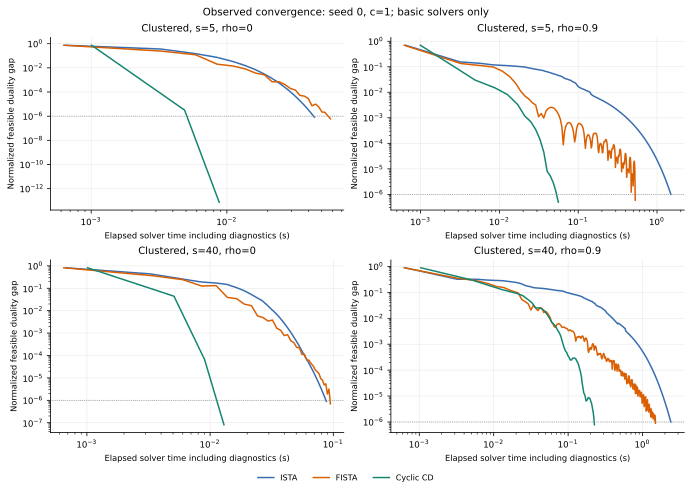
Table 1. Solve time in seconds at \( s=20 \), \( c=1 \), and the slowdown from \( \rho{=}0 \) to \( \rho{=}0.9 \).
| Method | Dispersed: \( \rho=0 \) | Dispersed: \( \rho=0.9 \) | Dispersed: Ratio | Clustered: \( \rho=0 \) | Clustered: \( \rho=0.9 \) | Clustered: Ratio |
|---|---|---|---|---|---|---|
| ISTA | 0.027 | 1.274 | 44.1 | 0.026 | 0.844 | 29.4 |
| FISTA | 0.032 | 0.707 | 22.4 | 0.029 | 0.515 | 17.1 |
| CD | 0.0032 | 0.070 | 17.9 | 0.0037 | 0.059 | 17.9 |
| skglm | 0.0069 | 0.020 | 3.2 | 0.0089 | 0.013 | 1.4 |
All 1440 synthetic solves reach \( G_{\mathrm{norm}}\le10^{-6} \), with median times over the full grid of 0.113 s for ISTA, 0.105 s for FISTA, 0.0089 s for CD, and 0.0073 s for skglm. Table 1 reports medians over 5 seeds, and its ratio column is the median over seeds of the \( \rho{=}0.9 \) time divided by the \( \rho{=}0 \) time. In Table 1 and Figure 1, ISTA is the most affected by correlation: at \( \rho=0.9 \) its time grows by a factor of 29–44, and its median iteration count rises from about 130 to 3915 in the clustered layout and 5985 in the dispersed layout. The roughly fivefold growth of \( L \) in Section 3.1 accounts for part of this slowdown, and worse conditioning near the optimum accounts for the rest. In the clustered layout, the condition number of the Gram matrix of the true support rises from 2.0 to 72.7. In the dispersed layout, this condition number stays near 2, and the slowdown coincides with many false selections of correlated variables, which lower F1 in Figure 2. FISTA is about 1.8 times faster than ISTA at \( \rho=0.9 \) in the dispersed layout and close to ISTA at \( \rho=0 \). The right column of Figure 1 shows nonmonotone fluctuations in its gap curve, consistent with its oscillating objective. CD time grows by a factor of about 18, since stronger coupling between coordinates at high correlation requires more epochs. skglm updates a few coordinates within its working set and applies extrapolation, and its time grows only by a factor of 1.4–3.2. The four methods return identical final supports on all 360 targets.
The iteration counts behind Table 1 show the convergence rate directly. For ISTA, moving \( G_{\mathrm{norm}} \) from \( 10^{-2} \) to \( 10^{-4} \) and from \( 10^{-4} \) to \( 10^{-6} \) takes nearly the same number of iterations in every setting, for example 2425 and 2440 in the dispersed layout at \( \rho=0.9 \). The gap therefore falls linearly. Under the \( O(1/k) \) bound alone, each factor of 100 would multiply the iteration count by 100. The linear rate of Section 3.2 predicts the count. With \( A \) the support of the fitted solution, \( (L/\mu_A)\ln100 \) gives 41 and 1905 iterations at \( \rho=0 \) and \( 0.9 \) in the clustered layout, against 40 and 1875 observed, and 40 and 2642 in the dispersed layout, against 40 and 2440. The dispersed case shows that the relevant curvature belongs to the selected set. Its true support keeps \( \mu \) near 0.7 at every \( \rho \), whereas the fitted support grows to about 56 correlated variables and \( \mu_A \) drops accordingly. CD also converges linearly, with 60 epochs per two decades in the clustered layout and 80–85 in the dispersed layout at \( \rho=0.9 \). For FISTA, the count grows from one pair of decades to the next. At \( \rho=0.9 \) in the clustered layout, its second two decades take 1805 iterations against 630 for the first, as its momentum coefficient approaches 1 and the iterates overshoot near the solution. Because ISTA already converges linearly, the advantage that FISTA holds in the worst case shrinks to the factor of 1.8 in Table 1.
Table 2. Real data tasks solved to \( G_{\mathrm{norm}}\le10^{-6} \) without a time limit. Iterations are epochs for CD and outer iterations for skglm.
| Method | UJI longitude regression: Iterations | UJI longitude regression: Time (s) | UJI longitude regression: Test MSE | UJI longitude regression: Nonzeros | Leukemia: Iterations | Leukemia: Time (s) |
|---|---|---|---|---|---|---|
| ISTA | 7200 | 23.72 | 922.2 | 333 | 2,685,115 | 513.9 |
| FISTA | 2895 | 9.45 | 922.2 | 333 | 30,455 | 5.75 |
| CD | 345 | 1.56 | 922.2 | 333 | 1600 | 0.313 |
| skglm | 14 | 0.97 | 922.2 | 332 | 26 | 0.045 |
Table 2 reports the real data results. UJI values are medians over 3 splits, and Leukemia values are medians of 3 repeats. All methods reach the target in every run. FISTA takes 6–18 times as long as CD, and skglm is about 7 times faster than CD on Leukemia. ISTA takes 2.5 times as long as FISTA on UJI and 89 times as long on Leukemia. On Leukemia, ISTA still selects 123 variables after 36,000 iterations, more than the 72 samples. \( X_A^\top X_A \) is then singular and \( \mu_A=0 \), so the linear rate of Section 3.2 applies only after the selected set shrinks toward the final 68 variables, and ISTA needs 2.7 million iterations. On UJI, all four methods give a test MSE of 922.2 with 332–333 nonzeros, and the nonzero counts still differ by one.
5.2 Solver Accuracy and Support Stability
Table 3. Number of trajectories, out of 240, whose support matches the \( 10^{-10} \) reference, and the median extra time to go from \( 10^{-4} \) to \( 10^{-6} \).
| Metric | FISTA | CD |
|---|---|---|
| Match at \( G_{\mathrm{norm}}\le10^{-2} \) | 132/240 | 133/240 |
| Match at \( G_{\mathrm{norm}}\le10^{-4} \) | 239/240 | 236/240 |
| Match at \( G_{\mathrm{norm}}\le10^{-6} \) | 240/240 | 240/240 |
| Extra time, \( 10^{-4}\to10^{-6} \) | 0.308 s | 0.009 s |
| Share of total time | 66.5% | 32.8% |
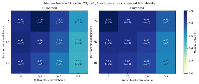
Table 3 counts each trajectory when it first reaches a given gap. The 5 mismatching trajectories at \( 10^{-4} \) involve 4 targets, all from settings with high correlation and dispersed support, and at \( 10^{-6} \) every trajectory is stable. Going from \( 10^{-4} \) to \( 10^{-6} \) takes about two thirds of the total FISTA time and one third of the total CD time. At \( 10^{-2} \), a further 9 FISTA and 11 CD trajectories select different variables from the reference while matching its TP, FP, and FN counts, so only a comparison of the selected variables reveals these cases.
Figure 2 shows statistical recovery at a common accuracy, using CD at \( c=1 \) and medians over 5 seeds. F1 generally decreases as \( \rho \) and \( s \) grow, and the two layouts fail in different ways. In the dispersed layout at \( \rho=0.9 \), recall stays at 1 while precision falls to 0.34–0.42: the Lasso spreads the signal over correlated variables in the same block and makes many false selections. In the clustered layout at \( \rho=0.9 \), recall falls to about 0.6, as only some of the true signals in a block are selected, in line with the grouping behaviour reported for the elastic net [2]. None of the 6 conditions at \( \rho=0.9 \) achieves exact recovery. The four methods return the same support in these conditions, so the recovery error comes from the Lasso estimator itself.
5.3 Support Differences at Equal Accuracy
On the 40 UJI semi-synthetic targets, sklearn and skglm both reach \( G_{\mathrm{norm}}\le10^{-10} \). For 10 targets, the two solutions agree exactly in coefficients, objective value, and support and signs under both thresholds. Under the main \( \tau \), the two supports give different F1 on 14 targets, with a maximum difference of 5.19 percentage points. With \( \tau=10^{-4} \) this rises to 18 targets. The largest coefficient difference in any coordinate between the two solutions is 0.952, the largest fit RMSE difference is \( 1.75\times10^{-10} \), and the objective difference is \( 4.4\times10^{-16} \), consistent with the theoretical result that Lasso fitted values are unique [3]. To separate implementation differences from degeneracy of the problem itself, we fix the implementation and change only the input column order.
Table 4. Column order experiment at \( G_{\mathrm{norm}}\le10^{-10} \) with 6 orders per target.
| Data | Solver | \( \tau \) | Targets | Changed | F1 \( > \)2pp | F1 \( > \)5pp | Max range |
|---|---|---|---|---|---|---|---|
| UJI | sklearn | \( 10^{-6} \) | 40 | 18 | 18 | 3 | 7.66 pp |
| UJI | skglm | \( 10^{-6} \) | 40 | 25 | 20 | 6 | 9.63 pp |
| UJI | sklearn | \( 10^{-4} \) | 40 | 20 | 20 | 5 | 7.66 pp |
| UJI | skglm | \( 10^{-4} \) | 40 | 23 | 16 | 4 | 11.11 pp |
| News | both | both | 8 | 0 | 0 | 0 | 0 |
| Gene | both | both | 8 | 0 | 0 | 0 | 0 |
All 784 calls in the column order experiment reach \( G_{\mathrm{norm}}\le10^{-10} \), and the 112 repeats match earlier results bit for bit. In Table 4, “Changed” counts targets whose support changes across orders, and the F1 columns count targets whose F1 range over the six outputs strictly exceeds 2 or 5 percentage points. The news and gene rows pool both implementations and both thresholds, which give identical results. As the table shows, on UJI the support changes with column order for 18 targets under sklearn and 25 under skglm, of which 18 and 20 have an F1 range above 2 percentage points. Treating the 4 targets of each seed as one independent unit, support changes occur in 7/10 seed blocks for sklearn and 9/10 for skglm. The effect is stronger in the clustered layout. Under skglm, the support changes on 15 of 20 clustered targets and 10 of 20 dispersed targets, with mean F1 ranges of 2.97 and 1.19 percentage points. This fits the idea that the allocation within a group is harder to determine when the group holds several true signals.
The target with the largest F1 range uses skglm on the clustered layout with mixed weak signals. Across the six outputs, F1 ranges from 0.727 to 0.824, the supports differ in at most 5 coordinates, the coefficient difference reaches 0.865, the fit RMSE difference is \( 1.4\times10^{-10} \), and the objective difference is \( 4.4\times10^{-16} \). For all news and gene targets, the largest coefficient difference is below \( 6\times10^{-10} \).
5.4 Nearly Proportional Feature Groups and Order Sensitivity
The UJI features are signal strengths of individual WiFi access points. After sampling 1000 rows, many access points are detected together in only a few rows, and their columns become nearly proportional, \( x_j\approx a_jx_{\mathrm{anchor}} \). Within such a group \( g \), the fitted values and the \( \ell_1 \) penalty stay nearly unchanged as long as the net group effect \( \theta_g=\sum_{j\in g}a_jw_j \) is fixed. The solution set is then nearly degenerate along directions inside a group, and the duality gap constrains these directions only weakly. Changing the column order changes the order in which coordinates are visited and how working sets are chosen, so the solver stops at a different point of the degenerate solution set. The location of the changed coordinates supports this explanation: all 27 changed coordinates under sklearn, and all 38 under skglm, lie in nearly proportional groups found by step 1 of the proposed method before fitting. After aggregating by net group effect, the two reference solutions agree on all 40 targets, with a maximum aggregated difference of about \( 4.5\times10^{-10} \). The 10 UJI targets on which the two references agreed exactly stay unchanged under every order.
The uniqueness condition for Lasso solutions explains why the news and gene data show no change under either implementation or threshold. Tibshirani [3] proved that the Lasso solution is unique when \( X_E \), with \( E \) the equicorrelation set of Proposition 1, has full column rank, which holds automatically when the columns of \( X \) are in general position. Two proportional columns have the same absolute correlation with any residual, so they enter \( E \) together and make \( X_E \) rank-deficient. The solution set then extends into a segment in the direction within the group, and the column order determines where on the segment the solver stops. UJI signal strengths are discrete, and undetected access points are recorded as a fixed value, so an access point detected in only one or two sampled rows becomes a duplicate column after standardization and falls into this case.
For the news and gene data, we apply step 2 of the proposed method to the two highly accurate solutions of each of the 36 confirmation targets per source, 144 outputs in total. Table 5 gives the results. Both full matrices are rank-deficient: the 58 news features contain linear dependencies, such as weekday dummies that always sum to 1, which gives a numerical rank of 56, and the gene matrix has \( p\gg n \) and a numerical rank of 71. All 144 submatrices \( X_{\bar E} \) have full column rank, with smallest singular values of at least 1.18, a clear margin from rank deficiency. The certificate therefore holds for every output, the solutions are unique, the solver converges to the same point from every column order, and the corresponding counts in Table 4 are 0.
Table 5. Uniqueness certificate of Section 3.3 for the news and gene confirmation targets.
| Quantity | News | Gene |
|---|---|---|
| Full matrix size | \( 1000\times58 \) | \( 72\times7129 \) |
| Rank of full matrix | 56 | 71 |
| Size of \( \bar E \) | 5–14 | 13–42 |
| \( X_{\bar E} \) of full rank | 72/72 | 72/72 |
| Min. \( \sigma_{\min}(X_{\bar E}) \) | 5.805 | 1.184 |
Table 6. UJI preprocessing comparison on 12 targets.
| Variant | Agree | F1 differ | Removed |
|---|---|---|---|
| Original | 2/12 | 7/12 | 0 |
| Exact dedup | 2/12 | 8/12 | 1–3 |
| Anchoring | 12/12 | 0/12 | 3–8 |
Table 7. Coefficients of three duplicate column groups under six column orders for the target with the largest F1 range.
| Order | \( w_a \) | \( w_{a’} \) | \( w_b \) | \( w_{b’} \) | \( w_c \) | \( w_{c’} \) | TP | FP | FN | F1 |
|---|---|---|---|---|---|---|---|---|---|---|
| Original | \( \mathbf{-0.865} \) | \( \mathbf{-6.1{\times}10^{-6}} \) | \( -2.8{\times}10^{-8} \) | \( \mathbf{-0.917} \) | \( \mathbf{-0.013} \) | 0 | 13 | 6 | 2 | 0.765 |
| \( \pi_1 \) | 0 | \( \mathbf{-0.865} \) | \( \mathbf{-1.1{\times}10^{-5}} \) | \( \mathbf{-0.916} \) | \( -2.7{\times}10^{-9} \) | \( \mathbf{-0.013} \) | 13 | 6 | 2 | 0.765 |
| \( \pi_2 \) | \( \mathbf{-0.865} \) | 0 | \( \mathbf{-9.4{\times}10^{-6}} \) | \( \mathbf{-0.916} \) | 0 | \( \mathbf{-0.013} \) | 14 | 5 | 1 | 0.824 |
| \( \pi_3 \) | 0 | \( \mathbf{-0.865} \) | 0 | \( \mathbf{-0.917} \) | \( \mathbf{-0.013} \) | \( -4.3{\times}10^{-8} \) | 12 | 6 | 3 | 0.727 |
| \( \pi_4 \) | \( \mathbf{-3.2{\times}10^{-6}} \) | \( \mathbf{-0.865} \) | \( \mathbf{-8.5{\times}10^{-6}} \) | \( \mathbf{-0.916} \) | \( \mathbf{-0.013} \) | \( -7.2{\times}10^{-9} \) | 14 | 6 | 1 | 0.800 |
| \( \pi_5 \) | \( \mathbf{-0.865} \) | \( -5.9{\times}10^{-9} \) | 0 | \( \mathbf{-0.917} \) | \( \mathbf{-0.013} \) | \( -8.1{\times}10^{-9} \) | 13 | 5 | 2 | 0.788 |
Table 7 lists every changed coordinate of the target with the largest F1 range. These coordinates come from three groups of duplicate columns, identical up to a relative residual of about \( 10^{-16} \). Here \( a \) and \( b \) are true variables, and \( a’ \), \( b’ \), \( c \), \( c’ \) have zero true coefficients. Bold entries satisfy \( |w_j|>\tau=10^{-6} \) and count toward the support, and absolute values below \( 10^{-9} \) are shown as 0. In group \( \{a,a’\} \), the coefficient \( -0.865 \) moves between the true variable \( a \) and its duplicate \( a’ \), and the coefficient sum of each of the three groups is the same in all six outputs. When the coefficient sits on \( a’ \), \( a \) counts as a miss and \( a’ \) as a false selection. The coefficient of the true variable \( b \) varies from the order of \( 10^{-5} \) down to 0, and whether it crosses the threshold \( \tau \) decides whether it enters the support. In the original order, \( a’ \) keeps a residual coefficient of \( -6.1\times10^{-6} \) and adds one false selection, while \( b \) stays below \( \tau \). Under \( \pi_2 \), \( a’ \) is zero and \( b \) crosses \( \tau \), which gives the highest F1. All differences in TP, FP, and FN across the six outputs come from the allocation within these three groups.
Table 6 tests merging nearly proportional columns across 3 seeds, two layouts, and two signal strengths. “Agree” counts targets on which the two reference solutions agree exactly, “F1 differ” counts targets whose two references differ in F1 under the main \( \tau \), and “Removed” counts deleted columns. Exact deduplication of the raw RSSI values removes 1 existing disagreement and introduces 2 new ones, raising the total to 8/12. Step 3 of the proposed method, which compresses each group from step 1 into a single anchor column, makes the two references agree exactly on 12/12 targets. Each design loses 3–8 original variables, and for 4 targets the removed columns include a true nonzero variable whose signal moves to the anchor column. In the merged coordinates, both implementations have an FN of 0, a mean FP of about 4.67, and no exact recoveries. Merging columns removes the order sensitivity, and the evaluation target changes accordingly from original variables to groups.
Output stability and recovery quality vary independently. The 36 external targets from each of the news and gene sources have identical support and F1 across both implementations and thresholds. The gene data have a median F1 of about 0.20 and no exact recoveries. On UJI, the 10 targets on which the two references agree have a mean F1 of about 0.829, against about 0.789 for the other 30. Since the stable subset has a higher mean F1, filtering tasks by stability inflates the reported recovery level.
6 Discussion and Limitations
When a design contains nearly proportional feature groups, the objective leaves the split of coefficients within each group free, and the solver path decides it. Recovery scores computed from a single solve then include a path component, which moved F1 by as much as 9.63 percentage points on our UJI tasks. The proposed procedure detects this case at low cost. The group scan takes at most 0.16 s per design in our experiments, and the certificate needs one solution and one SVD, against six full solves per target in the column order experiment. Reporting F1 on the full task set together with its range across column orders captures both the recovery level and the size of the path component.
The order effect appeared on UJI, where discrete signal strengths and rarely detected access points produce duplicate columns. Designs with many rarely nonzero discrete features are the next cases to test, together with experiments that separate the effects of coordinate order, working set selection, and rounding. The elastic net makes the objective strongly convex, and the group Lasso selects variables by group, so both remove this degeneracy at the model level and are natural candidates for comparison.
7 Conclusion
Under a common duality gap stopping rule, stronger feature correlation raised the Lipschitz constant and worsened the conditioning near the optimum. At \( \rho=0.9 \), ISTA, FISTA, and cyclic coordinate descent each took at least ten times as long as at \( \rho=0 \), and skglm took 1.4 to 3.2 times as long. ISTA and CD converged linearly near the solution, at rates set by the curvature on the selected support. Supports on the synthetic designs settled by a gap of \( 10^{-6} \). On UJIIndoorLoc, reordering the input columns still changed the selected variables at a gap of \( 10^{-10} \). Every change occurred within a nearly proportional feature group, and the outputs agreed once coefficients were summed by group. The proposed procedure checks uniqueness from one approximate solution. Its duality gap bound certified a unique solution for all news and gene outputs, and on UJI the detected groups moved the evaluation to the group level.
helped by GPT-6.1 sol/Astra and Claude Opus 5.5
References
- Robert Tibshirani. Regression Shrinkage and Selection via the Lasso. Journal of the Royal Statistical Society: Series B, 58(1):267–288, 1996.
- Hui Zou and Trevor Hastie. Regularization and Variable Selection via the Elastic Net. Journal of the Royal Statistical Society: Series B, 67(2):301–320, 2005.
- Ryan J. Tibshirani. The Lasso Problem and Uniqueness. Electronic Journal of Statistics, 7:1456–1490, 2013.
- Amir Beck and Marc Teboulle. A Fast Iterative Shrinkage-Thresholding Algorithm for Linear Inverse Problems. SIAM Journal on Imaging Sciences, 2(1):183–202, 2009.
- Badr Moufad, Pierre-Antoine Bannier, Quentin Bertrand, Quentin Klopfenstein, and Mathurin Massias. skglm: Improving scikit-learn for Regularized Generalized Linear Models. Journal of Machine Learning Research, 26(149):1–6, 2025.
- Martin J. Wainwright. Sharp Thresholds for High-Dimensional and Noisy Sparsity Recovery Using \( \ell_1 \)-Constrained Quadratic Programming (Lasso). IEEE Transactions on Information Theory, 55(5):2183–2202, 2009.
- Ankit Kumar, Sharmodeep Bhattacharyya, and Kristofer Bouchard. Numerical Characterization of Support Recovery in Sparse Regression with Correlated Design. Communications in Statistics – Simulation and Computation, 53(3):1504–1518, 2024.
- Joaquín Torres-Sospedra, Raúl Montoliu, Adolfo Martínez-Usó, Tomás J. Arnau, and Joan P. Avariento. UJIIndoorLoc. UCI Machine Learning Repository, 2014.
- Ingrid Daubechies, Michel Defrise, and Christine De Mol. An Iterative Thresholding Algorithm for Linear Inverse Problems with a Sparsity Constraint. Communications on Pure and Applied Mathematics, 57(11):1413–1457, 2004.
- Paul Tseng. Convergence of a Block Coordinate Descent Method for Nondifferentiable Minimization. Journal of Optimization Theory and Applications, 109(3):475–494, 2001.
- Jerome Friedman, Trevor Hastie, and Robert Tibshirani. Regularization Paths for Generalized Linear Models via Coordinate Descent. Journal of Statistical Software, 33(1):1–22, 2010.
- J. Kenneth Tay, Balasubramanian Narasimhan, and Trevor Hastie. Elastic Net Regularization Paths for All Generalized Linear Models. Journal of Statistical Software, 106(1):1–31, 2023.
- James Yang and Trevor Hastie. A Fast and Scalable Pathwise-Solver for Group Lasso and Elastic Net Penalized Regression via Block-Coordinate Descent. arXiv preprint arXiv:2405.08631, 2024.
- Quentin Bertrand and Mathurin Massias. Anderson Acceleration of Coordinate Descent. In Proceedings of AISTATS, PMLR 130, pages 1288–1296, 2021.
- Johan Larsson, Quentin Klopfenstein, Mathurin Massias, and Jonas Wallin. Coordinate Descent for SLOPE. In Proceedings of AISTATS, PMLR 206, pages 4802–4821, 2023.
- Olivier Fercoq, Alexandre Gramfort, and Joseph Salmon. Mind the Duality Gap: Safer Rules for the Lasso. In Proceedings of ICML, PMLR 37, pages 333–342, 2015.
- Eugene Ndiaye, Olivier Fercoq, Alexandre Gramfort, and Joseph Salmon. Gap Safe Screening Rules for Sparsity Enforcing Penalties. Journal of Machine Learning Research, 18(128):1–33, 2017.
- Iyad Walwil and Olivier Fercoq. The Smoothed Duality Gap as a Stopping Criterion. Mathematical Programming Computation, 17(4):653–697, 2025.
- Peng Zhao and Bin Yu. On Model Selection Consistency of Lasso. Journal of Machine Learning Research, 7(90):2541–2563, 2006.
- Jonathan W. Stallrich, Kade Young, Maria L. Weese, Byran J. Smucker, and David J. Edwards. An Optimal Design Framework for Lasso Sign Recovery. Journal of the Royal Statistical Society: Series B, 87(5):1457–1480, 2025.
- Stanislav Minsker and Yiqiu Shen. The Impact of Contamination and Correlated Design on the Lasso: An Average Case Analysis. Statistics & Probability Letters, 223:110417, 2025.
- Rares-Darius Buhai. Lasso and Partially-Rotated Designs. arXiv preprint arXiv:2505.11093, 2025.
- Huizhen Bu, Takuya Nagata, Kakeru Onodera, and Sumika Arima. Sparse Reluctant Interaction Modelling with Convex Hull Approximation—For Accurate Modelling of Highly Correlated Variables Based on Diverse Nearly Optimal Solutions. Journal of Japan Industrial Management Association, 73(4E):223–233, 2023.
- Alexander Bastounis, Felipe Cucker, and Anders C. Hansen. When Can You Trust Feature Selection? – I: A Condition-Based Analysis of LASSO and Generalised Hardness of Approximation. arXiv preprint arXiv:2312.11425, 2023.
- Alexander Bastounis, Felipe Cucker, and Anders C. Hansen. When Can You Trust Feature Selection? – II: On the Effects of Random Data on Condition in Statistics and Optimisation. arXiv preprint arXiv:2312.11429, 2023.
- Yingying Li and Stanley Osher. Coordinate Descent Optimization for \( \ell^1 \) Minimization with Application to Compressed Sensing; a Greedy Algorithm. Inverse Problems and Imaging, 3(3):487–503, 2009.
- Donghwa Kim, Jaewook Lee, and Chulhee Yun. Provable Benefit of Random Permutations over Uniform Sampling in Stochastic Coordinate Descent. In Proceedings of ICML, PMLR 267, pages 30480–30547, 2025.
- Asher Spector and Lucas Janson. Powerful Knockoffs via Minimizing Reconstructability. The Annals of Statistics, 50(1):252–276, 2022.
- Mahdi Nouraie, Connor Smith, and Samuel Muller. Stability Selection via Variable Decorrelation. Statistics and Computing, 36(4):160, 2026.
- Elaine T. Hale, Wotao Yin, and Yin Zhang. Fixed-Point Continuation for \( \ell_1 \)-Minimization: Methodology and Convergence. SIAM Journal on Optimization, 19(3):1107–1130, 2008.
- Todd R. Golub et al. Molecular Classification of Cancer: Class Discovery and Class Prediction by Gene Expression Monitoring. Science, 286(5439):531–537, 1999.
- Kelwin Fernandes, Pedro Vinagre, Paulo Cortez, and Pedro Sernadela. Online News Popularity. UCI Machine Learning Repository, 2015.